Peptide level intensity normalization across experiments

In this tutorial, we start with a simulated table of peptides, quantified across a set of experiments. We will add some extra noise and then perform normalization to correct for that noise.

import pandas as pd
import numpy as np
import matplotlib.pyplot as plt
from omicspylib.plots import plot_density

from omicspylib.datasets.peptides import PeptidesDataset

from omicspylib import __version__

print(f'omicspylib version: {__version__}')

omicspylib version: 0.0.7

The simulated dataset is loaded as a Pandas data frame. Peptide identifiers are under peptide_id column, protein identifiers under protein_id column and columns cX_repY represent measured peptides intensities/quantitative values.

data_df = pd.read_csv('data/peptides_dataset.tsv', sep='\t')
data_df.head(2)

	peptide_id	protein_id	c1_rep1	c1_rep2	c1_rep3	c1_rep4	c1_rep5	c2_rep1	c2_rep2	c2_rep3	c2_rep4	c2_rep5	c3_rep1	c3_rep2	c3_rep3	c3_rep4	c3_rep5
0	pept147	prot0	1740.912460	0.0	1393.260017	4685.874636	513.393605	502.109101	949.462139	0.000000	3006.548317	671.891115	4123.628101	11583.385623	3114.882410	2812.034141	2195.550530
1	pept424	prot0	3668.876134	0.0	0.000000	303.011791	1314.382432	404.828763	3723.604607	11838.405382	7586.141805	0.000000	336.363330	0.000000	200.425728	3891.630707	1395.146624

We will shift the measurements by a fixed value to make the effect of normalization more visible. First we transform the values to approximate normal distribution and then shift by a fixed value. Then we apply a mask to set to 0.0 cases with 0.0 initial value.

exp_col = [c for c in data_df.columns if '_rep' in c]
random_shift = np.random.uniform(0, 5, len(exp_col)).reshape(1, -1)
mask = data_df[exp_col] > 1

data_df[exp_col] = 2**(np.log2(data_df[exp_col]+1) + random_shift)
data_df[exp_col] *= mask
data_df.head(2)

	peptide_id	protein_id	c1_rep1	c1_rep2	c1_rep3	c1_rep4	c1_rep5	c2_rep1	c2_rep2	c2_rep3	c2_rep4	c2_rep5	c3_rep1	c3_rep2	c3_rep3	c3_rep4	c3_rep5
0	pept147	prot0	8207.742261	0.0	3340.489492	9174.312026	1135.664727	1636.533298	23932.710404	0.000000	12038.502978	2916.229804	105123.431332	11897.564858	30812.298059	26757.316943	38482.987426
1	pept424	prot0	17292.141906	0.0	0.000000	595.087184	2904.066879	1320.095946	93785.833003	23282.136174	30369.530123	0.000000	8598.300247	0.000000	1991.856161	37026.338229	24460.121563

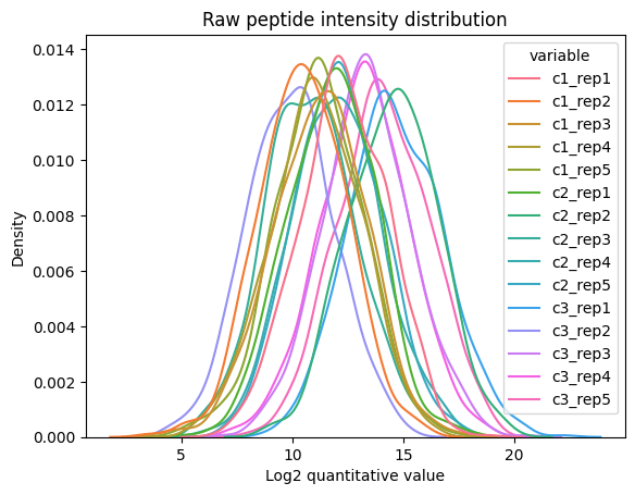
Then, we can create the PeptidesDataset object from the tabular data and visualize the peptide abundance distribution. There is an significant level of noise that needs to be corrected before attempting any comparison between the experimental conditions.

config = {
    # since we create a PeptidesDataset, id_col points to the peptide identifier column
    'id_col': 'peptide_id',
    # specify columns of the experimental conditions and their related experiments
    'conditions': {
        'c1': ['c1_rep1', 'c1_rep2', 'c1_rep3', 'c1_rep4', 'c1_rep5'],
        'c2': ['c2_rep1', 'c2_rep2', 'c2_rep3', 'c2_rep4', 'c2_rep5'],
        'c3': ['c3_rep1', 'c3_rep2', 'c3_rep3', 'c3_rep4', 'c3_rep5'],
    },
    # specify the column name of the protein identifier, so that you can calculate protein abundance values in the end
    'protein_id_col': 'protein_id',
}
raw_pept_dset = PeptidesDataset.from_df(data_df, **config)

plot_density(
    dataset=raw_pept_dset,
    log_transform=True,
    xlabel='Log2 quantitative value',
    ylabel='Density',
    title='Raw peptide intensity distribution')
plt.show()

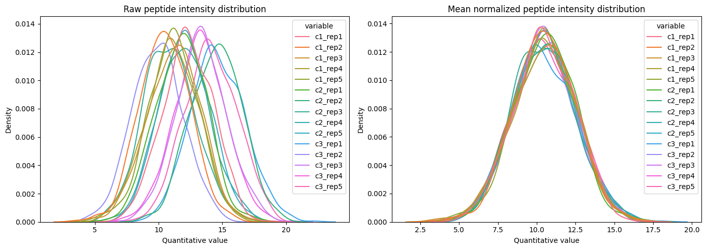
To normalize the dataset, call the .normalize method. Currently, only normalization to the mean value of the peptide distribution is supported with extra options (see documentation).

When using the default values, the steps during the normalization include:

1. Find the experiment with the most records and consider reference.

2. Calculate mean experiment intensity and the difference from reference.

3. Shift each experiment’s intensity by the difference with reference.

Optionally, you can set reference experiment with the ref_exp argument, or a reference experimental condition to automatically pick the reference using the ref_condition argument.

Note that normalization is done on normally distributed data. For this, you need to do any related transformation before and after that step. For example, you might use Log2 transformation before the normalization and back transform to the original scale afterward.

# normalize the dataset
norm_pept_dset = raw_pept_dset\
    .log2_transform()\
    .normalize(method='mean')\
    .log2_backtransform()

# plot before and after normalization
fig, ax = plt.subplots(1, 2, figsize=(14, 5))
plot_density(
    dataset=raw_pept_dset,
    log_transform=True,
    title='Raw peptide intensity distribution',
    ax=ax[0])

plot_density(
    dataset=norm_pept_dset,
    log_transform=True,
    title='Mean normalized peptide intensity distribution',
    ax=ax[1])
plt.tight_layout()
plt.show()
# pept_df

Finally, use the normalized peptide values to calculate protein abundance as the sum of peptide abundance values, and continue your analysis pipeline.

proteins_dset = norm_pept_dset.to_proteins()
prot_df = proteins_dset.to_table()
prot_df.head(2)

	c1_rep1	c1_rep2	c1_rep3	c1_rep4	c1_rep5	c2_rep1	c2_rep2	c2_rep3	c2_rep4	c2_rep5	c3_rep1	c3_rep2	c3_rep3	c3_rep4	c3_rep5
protein_id
prot0	31591.837412	13990.809596	12324.678681	22023.734731	14694.277136	14427.119874	45839.563199	59211.802455	23086.862365	22146.803428	31218.149389	28015.428540	54998.218152	97102.374965	15396.715568
prot1	34552.115281	69917.183544	41572.100739	7044.607483	8136.515734	8993.403622	26526.500835	21703.822784	31303.386236	49314.501471	21025.427164	53153.792459	6947.123719	19045.165135	52347.668785