Hierarchically clustered heatmaps

In this tutorial, we start with a proteins dataset and perform hierarchical clustering on the data. Then plot a heatmap where we overlay the clustering tree and color the entries based on their group. This implementation uses internally the clustermap plotting function from the Seaborn library.

from omicspylib.analysis.clusters import HierarchicallyClusteredHeatmap
import pandas as pd
import matplotlib.pyplot as plt
from omicspylib import ProteinsDataset
from omicspylib import __version__

print(f'omicspylib version: {__version__}')

omicspylib version: 0.0.8

Load our proteins table containing the protein identifier and the quantitative value per experimental condition.

data = pd.read_csv('data/protein_dataset.tsv', sep='\t')
data.head(2)

	protein_id	c1_rep1	c1_rep2	c1_rep3	c1_rep4	c1_rep5	c2_rep1	c2_rep2	c2_rep3	c2_rep4	c2_rep5	c3_rep1	c3_rep2	c3_rep3	c3_rep4	c3_rep5
0	p0	1748947.964	2655665.55	1812807.047	3179830.747	3002006.748	0.000	1357720.520	0.000	2087116.684	0.000	2558776.479	2655657.487	2115434.782	2889376.029	0.0
1	p1	1689613.957	0.00	1953790.640	2447525.246	2877005.859	1438315.297	1198347.576	1864606.985	0.000	1414141.418	0.000	3070691.996	3149289.453	0.000	2264704.9

To create the heatmap, you need to keep in the table only the quantitative values. The unique identifiers (protein id in this case) should be placed in the index.

hm_inputs = data.set_index('protein_id')
hm_inputs.head(2)

	c1_rep1	c1_rep2	c1_rep3	c1_rep4	c1_rep5	c2_rep1	c2_rep2	c2_rep3	c2_rep4	c2_rep5	c3_rep1	c3_rep2	c3_rep3	c3_rep4	c3_rep5
protein_id
p0	1748947.964	2655665.55	1812807.047	3179830.747	3002006.748	0.000	1357720.520	0.000	2087116.684	0.000	2558776.479	2655657.487	2115434.782	2889376.029	0.0
p1	1689613.957	0.00	1953790.640	2447525.246	2877005.859	1438315.297	1198347.576	1864606.985	0.000	1414141.418	0.000	3070691.996	3149289.453	0.000	2264704.9

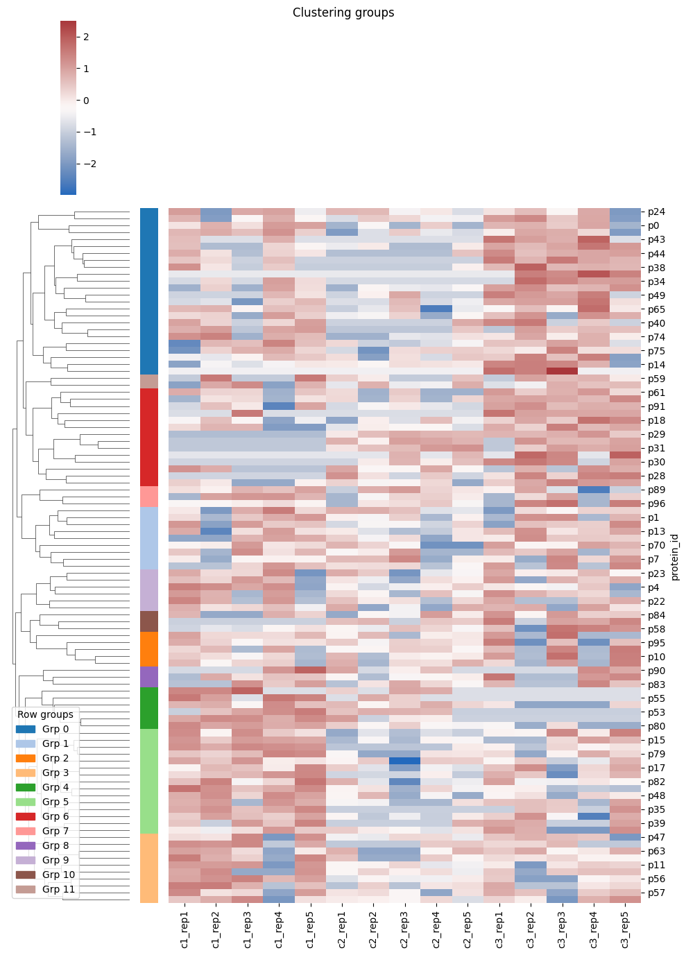
To create the heatmap use the HierarchicallyClusteredHeatmap object. It will return a filtered version of the data, a plot object and two lists with the group number of the rows and columns. Returned data might have less rows than the provided dataset, based on the filtering applied. For example, you might want to consider only the cases identified across 5 or more experiments. The unique row identifier is still in the index, so you can join back to the original dataset.

heatmap = HierarchicallyClusteredHeatmap(min_frequency=5, n_row_clusters=10, n_col_clusters=3)

result = heatmap.eval(data=hm_inputs, figsize=(5, 8))
plt.show()

print(f'N. rows before: {hm_inputs.shape[0]}')
print(f'N. rows after: {result.filtered_data.shape[0]}')
print(f'Row group idx: {result.row_groups}')
print(f'Col group idx: {result.col_groups}')

N. rows before: 100
N. rows after: 97
Row group idx: [0, 1, 0, 1, 2, 1, 0, 1, 3, 0, 4, 3, 5, 1, 0, 3, 6, 3, 6, 7, 3, 8, 2, 2, 0, 6, 6, 6, 6, 6, 6, 0, 3, 0, 0, 0, 3, 0, 6, 3, 0, 0, 0, 6, 3, 3, 0, 4, 3, 5, 5, 5, 5, 3, 3, 6, 6, 1, 6, 0, 3, 3, 0, 4, 3, 3, 3, 1, 3, 3, 0, 0, 0, 0, 0, 3, 3, 5, 2, 3, 8, 0, 6, 2, 2, 6, 7, 8, 6, 3, 3, 1, 4, 7, 9, 4, 1]
Col group idx: [0, 0, 0, 1, 0, 0, 0, 0, 0, 0, 2, 2, 2, 2, 2]

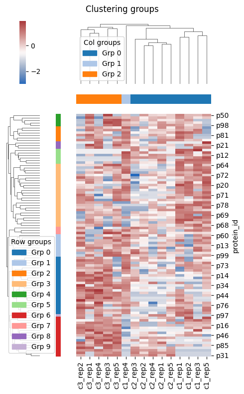
Alternatively your data are wrapped around a ProteinsDataset object, you can extract the table and proceed.

conditions = {
    'c1': [f'c1_rep{i+1}' for i in range(5)],
    'c2': [f'c2_rep{i+1}' for i in range(5)],
    'c3': [f'c3_rep{i+1}' for i in range(5)],
}
dataset = ProteinsDataset.from_df(data, id_col='protein_id', conditions=conditions)
data_in = dataset.to_table()

heatmap = HierarchicallyClusteredHeatmap(n_col_clusters=None)
result = heatmap.eval(data=data_in)
# plt.savefig('my-plot.png')  # save as image
# plt.savefig('my-plot.pdf')  # save as vector-based image
plt.show()